
PHYS 460 Class Info
TEST 1 will be Tues. Oct 4 and will cover Chap 1 through Chap 2.5. Bring your book and a calculator.
TEST 2 will be Thurs Nov 17. Chap 2.5 through the material in Sec 4.1. Remember there was a lot of material not in Chap 4 of the book that was covered in class. See the Chap 4 notes below to see what was covered. Bring your book and a calculator.
FINAL will be Thurs Dec 15 from 7-9 pm. The final will be comprehensive.
The text book for the class is Introduction to Quantum Mechanics 2nd Edition by David J. Griffiths. The tests are open textbook so you must have access to a physical copy (not electronic because you can't have open laptop during test).
Errata from Griffiths web page: Errata 1 ; Errata 2; Errata 3
We will cover most of Part 1 of Griffiths (Chapters 1-5) and possibly part of Chapter 12. Course description.
Syllabus
Office hours: Monday 4-5, Tuesday 10-11 (Contact me by email if you want to arrange a special time.)
Homework will be due by midnight on Tuesdays. You must show enough work on the homework so the grader can understand what you're doing.
Class
Notes
Chap 1; Chap 1 (extra) ; Chap 2; Chap 2
eigenstates.pdf; Chap2eig_state.ppt ; Chap2group_vel.ppt
; Chap2scattering.ppt
; Chap 3; Chap 4; Legendre Polynomials, Associated Legendre Polynomials, Spherical Harmonics
Spherical Bessel Functions, Radial energies/wave functions ; Chap 5
Homework
HWK 1 (Due Tues Aug 30, [Orals this week] 7 problems total): Problems 1-6 are Griffiths Chap 1 probs 1, 2, 3, 4, 5, 7
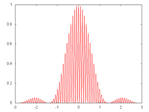
Problem 7 is numerical: Define k = 15 pi and dk = pi/3. For the range x = -3 to x = 3, PLOT the SQUARE of each of the four functions:
f1(x) = cos(k x)
f2(x) = [cos(k x) + cos((k+dk) x) + cos((k-dk) x)]/3
f3(x) = [cos(k x) + cos((k+dk) x) + cos((k-dk) x) + cos((k+2dk) x) + cos((k-2dk) x)]/5
f4(x) = [cos(k x) + cos((k+dk) x) + cos((k-dk) x) + cos((k+2dk) x) + cos((k-2dk) x) + cos((k+3dk) x) + cos((k-3dk) x)]/7
(These look complicated but you should see the pattern.) These functions oscillate very fast so you might want to have a small spacing of points in x. What do these functions inform you about an "uncertainty relation" between the spread in k and the spread in x? (This last question is squishy so a qualitative answer will suffice.)
You can check by comparing to the plot below which is the f4(x) but has k = 11 pi and dk = pi /5.0
HWK 2 (Due Tues Sep 6, 7 problems total): Griffiths probs 1.9, 1.16, 1.17, 2.1, 2.2, 2.3
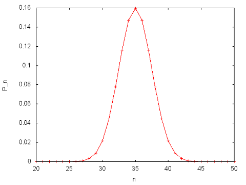
Problem 7 is numerical: An electron is in an infinite square well with walls at x = 0 and x = L = 100 a (where a is the Bohr radius). The wave function (Eq. 2.15 Griffiths) at t=0 has cn = A exp(-{[n-30]/4}2) exp(i (n pi/L) x0) with x0 = L/2 = 50 a. (a) Give the numerical value of A to 6 significant digits. (b) Plot the probability, Pn, that a measurement of the energy will give the value En vs. n.
For the case, cn = A exp(-{[n-35]/5}2) exp(i (n pi/L) x0), I found A = 0.39947079 and the plot looks like
HWK 3 (Due Tues Sep 13, [Orals this week] 7 problems total): Griffiths 2.5, 2.6, 2.7, 2.9, 2.15, 2.16
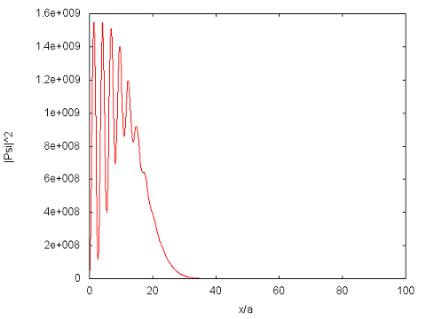
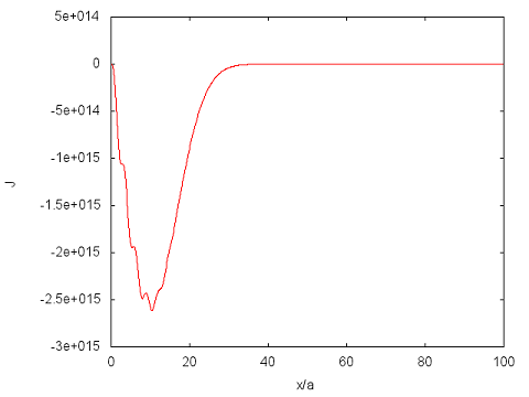
Problem 7 is a continuation of the numerical problem from HWK 2. Use the coefficients from HWK2 prob 7 to compute and plot |Psi (x,t)|2 and J(x,t) at times t = 0, T/4, T/2, (3/4)T, and T where T = L/v with v = 30 pi hbar/(L M). M is the mass. Interpret your results.
For the case, cn = A exp(-{[n-35]/5}2) exp(i (n pi/L) x0), the plots at t = 0.4T where T = L/v with v = 35 pi hbar/(L M) are:
HWK 4 (Due Tues Sep 20, 7 problems total): Griffiths probs 2.17, 2.10, 2.11, 2.12, 2.13, 2.14
Problem 7 is numerical: Plot the n=14 harmonic oscillator wave function for the case where the scale factor sqrt(m omega/hbar) = 1. On the same graph plot the two curves F(x) = +/- psi(0) * sqrt(p(0)/p(x)) where p(x) is the classical momentum at position x for the energy of the n=14 state. (Note p(x) is only defined in the classically allowed region.) Why do you expect the wave function to oscillate with an amplitude proportional to 1/sqrt(p(x))? Once you have your code working for n=14 you might try calculations for other n. Unless you're really careful in how you program, your code will give you garbage starting at some large n.
Make sure your graph doesn't have ranges so big you can't actually see the plot. Below is my calculation for n=12 (not 14 like I'm asking you). In my program, I computed the 14th hermite polynomial using Eq. 2.87. My code look liked this for each value of xi
herm[0] = 1.0 ; herm[1] = 2.0*xi ;
for(j = 1 ; j < nfin ; j++) herm[j+1] = 2.0*xi*herm[j] - 2*j*herm[j-1] ;
psi = coef*herm[nfin]*exp(-0.5*xi*xi) ;
HWK 5 (Due Tues Sep 27, [Orals this week] 7 problems total): Griffiths 2.20, 2.21, 2.22, 2.23, 2.25 (hint: integrate by parts once to evaluate <p^2>), 2.34
Problem 7 is numerical: Reproduce Fig. 2.6 for E = 0.495 hbar omega and 0.505 hbar omega (use the Fig. 2.6 to check your program). For the case of E = 0.495 hbar omega give the numerical values of an for 0 through 10 starting with a0 = 1 and a1 = 0 (give your numbers to 5 sig figs). For example, a2 = 5.0000E-3. (For your own intellectual curiosity, you might repeat with E closer to (1/2) hbar omega to see how non-eigenstates become eigenstates as E goes to an eigen-energy.)
HWK 6 (Due Thur Oct 13 7 problems total): Griffiths 2.29, 2.32, 3.3, 3.5, 3.7, 3.10
Problem 7 is numerical and is to find the ground state energy to 4 significant digits for a particle in a finite well. Use Eq. 2.154. Use a = 1 nm, M = 1E-30 kg, hbar = 1.0545E-34 J s, and V_0 = b (hbar hbar/[2 M (2 a) (2 a)]) where b = 1/2. (Use exactly these values to the digits shown otherwise you will get a different answer.)
(My algorithm used the fact that K - l tan(l a) > 0 if E is less than the correct energy and is <0 if E is greater than the correct energy but less than the value that gives l a = pi/2 (see Fig 2.18). So I start with one energy, E1, lower and one energy, E2, higher than the correct energy. You know E > -V0 and you know E < the case l a = pi/2 so choose these for E1 and E2. I then compute the average. I then compute K - l tan(l a) at this value. If it is > 0 then that E must be less than the correct energy so swap it for E1, else swap it for E2. Every iteration decreases the difference, E2-E1, by a factor of 2.)
Once you've solved this, you can think about how to get the odd eigenstates and the even higher energy states.
You can ask me about other algorithms that converge faster...
e1 = -v0 ;
e2 = (hbar*hbar*0.5/M) *(pi*0.5/a)*(pi*0.5/a) - v0 ;
if(e2 > 0.0) e2 = 0.0 ;
while((e2-e1) > (-e2-e1)*1.e-8)
{
etrial = 0.5*(e1 + e2) ;
k = sqrt(-2.0*M*etrial)/hbar ;
l = sqrt(2.0*M*(etrial+v0))/hbar ;
ftrial = k - l*tan(l*a) ;
print out the etrial and ftrial to make sure ftrial is going to 0
if(ftrial > 0.0) e1 = etrial ;
else e2 = etrial ;
}
To test your code, I give E for other values of b:
b = 0.1 gives E = -3.363340E-24 J
b = 0.2 gives E = -1.303859E-23 J
b = 0.3 gives E = -2.846671E-23 J
HWK 7 (Due Tues Oct 18, [Orals this week on HWK 6 and 7] 4 problems total): Griffiths 3.13, 3.14, 3.31 (the Virial Theorem is very famous and very useful)
Problem 4 is numerical and shows how
F(x,y) = psi_1(x) psi_1(y) + psi_2(x) psi_2(y) + psi_3(x) psi_3(y) + ...
converges to the Dirac delta function: delta(x - y).
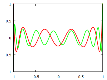
For the infinite square well with a = 1 nm and y/a = 0.4, plot F(x,y) vs. x/a for a sums that stop at n = 10, 20, 40, and 80. (Make sure you have enough x-points to trace out the curve.) There are other ways of doing the sum that converge faster to a delta function; ask me if you're interested. My answer for sums that stop at 10 (red) and 20 (green) are:
The oscillations are an example of Gibbs' phenomenon.
HWK 8 (Due Tues Oct 25, 7 problems total): Griffiths 3.16, 3.17, 3.21, 3.22, 3.28, 3.35,
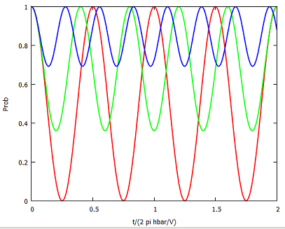
Problem 7 is numerical. You have a 2X2 Hamiltonian with elements
H11 = E1 = - H22 (note the minus sign for H22) and H12 = H21 = V
Plot the probability to be in state 1 as a function of time from 0 to 4 pi hbar/V when the wave function is 100% in state 1 at t=0. Do 5 cases: E1 = 0, E1 = V/4, E1 = V/2, E1 = V, E1 = 2 V. You can put them all on the same graph but clearly state which one is which. For comparison, the graph below is for E1 = 0 (red), E1 = 3 V/4 (green) and E1 = 3 V/2 (blue).
HWK 9 (Due Tues Nov 1, 7 problems total [Orals this week]): Griffiths 4.1, 4.2, 4.38
Prob 4: For the 2D Harmonic oscillator with potential
V(rho) = (1/2) M omega2 rho2
(a) Show that separation of variables in cartesian coordinates turns this into two one-dimensional oscillators, and exploit your knowledge of the latter to determine the allowed energies. (b) Determine the degeneracy d(n) of En.
Prob 5: Use the results from Prob 4. (a) Is the ground state also an eigenstate of Lz? (b) Are the two eigenstates with an energy increased by hbar omega from the ground state, eigenstates of Lz? (c) Are the three eigenstates with an energy increased by 2 hbar omega from the ground states, eigenstates of Lz? Show work. (Hint: Just do it: use the states in terms of x,y [combine the two exponentials into a function of rho] and the differential form for Lz OR write Lz in terms of ladder operators and use the algebraic method.)
Prob 6: (a) Give the superposition of the two eigenstates in (5b) that ARE eigenstates of Lz. Give their eigenvalues. Make sure they are normalized. (b) Give the superposition of the three eigenstates in (5c) that ARE eigenstates of Lz. Give their eigenvalues (you should find -2 hbar, 0 hbar, and 2 hbar). Make sure they are normalized. (Hint: See hint for Prob 5 and write the
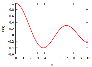
Prob 7 is numerical: The 2D Schrodinger equation for V=0 can be written as
-d2F(s)/ds2 - (1/s)dF(s)/ds + (m2/s2) F(s) = F(s)
where s = k rho. Determine what k is in terms of E, hbar, M, etc. For m=0, write F(s) as a power series in s. Give the recursion relation that lets you get cn from cn-1 and cn-2. Give the coefficient of each power as a column of numbers starting with c0 = 1 up to n=20 using 6 significant digits. A plot of F(s) is below which might help you check your coefficients.
Snippet of code to compute F(s) from cn
for(j = 0 ; j < 1000 ; j++)
{
s = j*0.01 ;
dum = 1.0 ;
f = 0.0 ;
for(n = 0 ; n < 51 ; n++)
{
f = f + coe[n]*dum ;
dum = dum*s ;
}
print out s, f
}
Plot of F(s):
HWK 10 (Due Tues Nov 8): Griffiths 4.3, 4.4, 4.5, 4.6, 3.39(a&b only) (note Chap 3!), 4.56(a only)
Prob 7 is numerical: Plot the L=20, 25, and 30 Legendre Polynomials. The recursion relation of Legendre Polynomials might be useful

My coding looks like this:
for(jx = -100 ; jx <= 100 ; jx++)
{
x = 0.01*jx ;
p[0] = 1.0 ;
p[1] = x ;
for(n = 1 ; n < 50 ; n++)
{
p[n+1] = ((2.0*n+1.0)*x*p[n] - n*p[n-1])/(n+1.0) ;
}
print out the appropriate info
}
The plot for L=10 and 15 looks like:
HWK 11 (Due Tues Nov 15): Griffiths 4.7, 4.8, 4.9, 4.39, 4.40, 4.41(a&b only, for b use the nr = 0, L=1, m=1 state of the 3D Harmonic oscillator)
Problem 7 is numerical: For the potential in Prob. 4.9, find the ground state energy for the case V_0 = 1.4 pi2 hbar2/(8 M a2). Give your answer as
E = -f pi2 hbar2/(2 M a2)
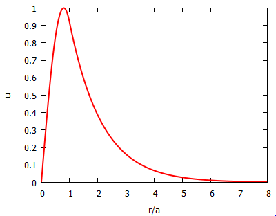
and give f to 4 significant digits. Make sure to show your algorithm and code. Plot your u(r) wave function (don't need to normalize) as a function of r/a.
For the case where the potential has V_0 = 1.9 pi2 hbar2/(8 M a2), I found f = 7.6396E-02 and the plot below:
HWK 12 (Due Tues Nov 29): Griffiths 4.10, 4.11, 4.13, 4.14
HWK 13 (Due Tues Dec 6 [Orals this week]): Griffiths 4.19, 4.20, 4.22, 4.24, 4.27, 4.33
Problem 7: Construct the spin matrices (Sx, Sy, Sz) for a particle of spin 3/2. (Hint: How many eigenstates of Sz are there? Determine the action of Sz, S+, and S- on each of these states. Follow the procedure used for spin 1/2.) Use these matrix representations to compute the commutator [Sx, Sy]. Also show that the representation gives the correct S2.
Tests/Solutions