A Brief Overview of Maple V
with Sample Applications to Elementary Physics

Software packages like Maple are called Computer Algebra Systems because they can manipulate symbolic information in ways that let a user obtain analytic solutions to many kinds of pure and applied mathematics problems. Since (some) humans can do this sort of thing themselves, what makes Computer Algebra Systems interesting is the speed and reliability with which they perform such manipulations. It will surprise no one to hear that this power can be put to good use in physics.

Today, Computer Algebra Systems are much more than the collections of symbolic manipulation routines they once were, and their new capabilities only increase their value to physics students and professionals. These capabilities include sophisticated tools for numeric computation and graphics as well as a user interface that supports not only computation but also the production of documents reporting computations and their results. This document is a Maple worksheet.

Getting Started

When you double-click on the Maple icon (Wmaple32 on PCs, Maple(FPU) on Macs or Maple(PPC) on Power Macs) or enter xmaple at the prompt in an XWindows session a window displaying three control bars, a status bar and a blank Maple worksheet opens.

The menu bar appears at the top of the window. Menus which drop down when you click on File or Edit provide access to operations like Opening, Saving and Printing worksheets; Copying, Cutting and Pasting and Exiting Maple. The tool bar, just below the menu bar, has button shortcuts to some of these and to other common operations. Just below it, control buttons and the information displayed on the context bar vary depending on whether you are working on text, Maple input or various types of Maple output. The status bar appears at the bottom of the Maple window.

The blank worksheet is displayed in the space between the context and status bars. The cursor blinks to the right of the prompt, >, in the worksheet's upper lefthand corner. This prompt marks the beginning of a Maple input region. Maple is waiting for an expression to evaluate.

Maple expressions can represent mathematical objects like numbers and functions and can invoke Maple commands that manipulate such objects or create special types of output from them, graphs for example. They can also define procedures (programs) that add new capabilities to the Maple system.

When Maple evaluates an expression the result is stored and can be displayed in an output region inserted into the worksheet beneath the input region containing the expression. The trick, of course, is to know what expressions to enter and evaluate so that Maple's output provides answers to questions of interest to you (or to your instructor).

A lot of analysis and problem solving can be done with fairly simple and intuitive types of Maple expressions. For example, it is quite clear from

> 3*6 + 4^2/(3 - 1);

that arithmetic expressions are entered using the usual computerish symbols, that the usual rules of precedence apply and that those rules can be overridden by using parentheses.

Additional examples of computations done by evaluating Maple expressions will be discussed shortly but, first, notice the semicolon that marks the end of the expression above. Since almost any combination of symbols constitutes a conceivable Maple expression and since expressions can run on for several lines you must mark their ends. The only way for Maple to know that your expression is complete is for you to mark the end of it with a semicolon or a colon. If you use a colon, Maple evaluates the expression, stores the result but does not display it. This is useful when you need but do not want to see complicated intermediate results when problem solving with Maple.

To have Maple evaluate or reevaluate an expression simply hit the <Enter> key when the cursor is in the input region containing it. If the worksheet contains input regions following that one, Maple will put the cursor in the next one when it is ready to accept more input. Otherwise, it will put the cursor in a new input region it creates at the end of your worksheet.

To convert an input region into a text region in which you can write explanatory comments simply click the T button on the tool bar when the cursor is in the region. The usual word processing tools are available to you in text regions. To toggle a text region back into an input region click the Sigma button on the tool bar. To insert a new input region beneath the region containing the cursor click the [> button on the tool bar.

There is space here to demonstrate only a few basic types of computation that can be done by evaluating Maple expressions. However, the examples in the remainder of this section do illustrate things a new user should try, offer an opportunity to suggest ways of avoiding the few pitfalls that can frustrate such users and provide some context for the Maple applications presented in the next section.

The output Maple returns after evaluating this arithmetic expression may surprise you.

> 3*6 + 4^2/3 - 1;

Maple returns this rational representation of the result because it is exact. If you want the useful, but usually approximate, floating-point representation of a number, you must ask Maple for it. You can do so explicitly or implicitly.

> evalf(3*6 + 4^2/3 - 1); 3*6.0 + 4^2/3 - 1;

The first of these expressions invokes Maple's evalf command which forces evaluation to floating point. The second demonstrates that floating point computation is generally "contagious". Once a floating point number, in this case 6.0, appears in an expression Maple generally uses floating point arithmetic to evaluate the entire expression.

The following examples illustrate some of Maple's other arithmetic capabilities.

> sqrt(2); arctan(sqrt(2.0)); Pi; evalf(Pi,50); cos(Pi/4);

> evalc(ln((1+I)/sqrt(2))); evalf(ln((1+I)/sqrt(2)));

You see that Maple knows about familiar functions and certain special constants like and i and that Maple's default floating point accuracy of 10 significant digits can be increased or decreased as needed.

Note well that Maple is case sensitive. It matters, for example, that the P in Pi is capitalized!

To see documentation on a Maple command like evalf or evalc you need only enter its name after a question mark in an input region and hit <Enter>.

> ?evalf

If you scroll to the bottom of the window that opens, you will usually find examples demonstrating the command's use. You can also find information on various Maple features in this Help System. For example, enter ?inifcn into an input region and hit <Enter> to see a list of the functions Maple knows about when you start it. Click Help on the menu bar and then Using Help for more on what the Help System can do for you.

Symbolic Maple expressions are often used to represent functions and equations involving them. In these examples x and y appear as variable names.

> 7*x^2*exp(x/2)*sin(x); 27*x*y+x^2/y^3; tan(y)=sqrt(x-y^2)/y;

Evaluating the following expressions assigns values to the variables f and z.

> f := 7*x^2*exp(x/2)*sin(x); z := 2;

A variable can be assigned any Maple expression as a value, and once a value is assigned to a variable its name evaluates to that value. Thus, f is now a convenient name for the expression and the value 2 is automatically plugged in for z when expressions involving that variable are evaluated. For example,

> Int(f,x=0..Pi)=int(f,x=0..Pi); 9*z^4 - 2*z;

Such full evaluation is obviously convenient, but it does create a pitfall. Imagine that you assign a value to a variable, say z, as you begin work on a new worksheet. If you use the variable z later in your Maple session having forgotten that it has the value you assigned it earlier, you will be surprised and confused by the results Maple returns for your expressions involving z. Note that this will be the case even if you have deleted all earlier references to z by editing you worksheet!

There are a couple of lessons here. First, when using Maple you must keep its internal state in mind. This includes variable values that you have assigned. Second, you must construct a worksheet with care if you want its appearance to reflect the evolution of Maple's state as it was being constructed.

To unassign a variable's value evaluate expressions like

> z := 'z';

which assign a variable's name to be its value, the normal state of affairs for free variables. Use ?quotes to access the Help System documentation on the use of quotation marks in Maple.

The following examples illustrate a few simple symbolic computations.

> expand((x+1)^2*(x-1)); expand(sin(a+b));

> factor(x^3+x^2-x-1); combine(sin(a)*cos(b)+cos(a)*sin(b));

> solve(x^2+7*x-2,x); subs(x=y*sin(phi), x^2+7*x-2);

> diff(f,x); series(tan(sin(x)),x=0);

> int(f,x);

> DE := t*diff(y(t),t)+2*y(t)=sin(t); dsolve(DE,y(t));

The Help System includes documentation on and examples demonstrating the use of the commands that appear in these expressions. It also includes documentation on and examples illustrating the use of these other useful commands: collect, convert, limit, simplify, normal, rhs, lhs, numer, denom, fsolve and dsolve[numeric]. Note that the last two of these are designed to find approximate answers to problems that do not admit analytic solutions. Here is an example,

> fsolve(cos(x)=x,x);

This overview of basic Maple use concludes with a brief look at Maple graphics. Only the basic plot command is demonstrated here. For information on the many commands that create 2- and 3-dimensional plots and animations click Help on the menu bar, click Contents, click the + button by Graphics and follow the hypertext links that appear.

In its simplest form the plot command takes two arguments, an expression representing the function of a single variable whose graph is to be drawn and an equation defining the range of the independent variable which the graph is to show.

> plot(tanh(x), x=-5..5, color=black);

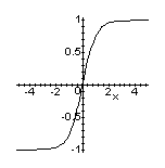
Notice how a..b is used to indicate a range in Maple. Use ?plot[options] to access the Help System documentation on optional arguments, like the third one in the example above. These are used to control the appearance of plots and can be a necessity when plotting a function on a domain in which it is singular. For example,

> plot(tan(x), x=-Pi..Pi, -10..10, discont=true, color=black);

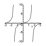
These final examples demonstrate ways of superimposing graphs on a single plot.

> plot({BesselJ(1,x), sin(x)}, x=0..4*Pi, color=black);

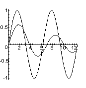
The expression {BesselJ(1,x), sin(x)} used in this command is a set of Maple expressions. In a similar vein, [BesselJ(1,x), sin(x)] is a list of expressions and BesselJ(1,x),sin(x) is a sequence of expressions. For information on these compound data types use ?sequence and ?set or ?list to access the relevant Help System documentation. Like plot, many Maple commands distribute over sequences, sets or lists of expressions.

The display command from the plots package also superimposes plots. However, it does so in a way that lets you control the appearance of each graph superimposed.

> with(plots):
> p1 := plot(BesselJ(1,x), x=0..4*Pi, color=blue):
> p2 := plot(sin(x), x=0..4*Pi, linestyle=2, color=black):
> display({p1,p2});

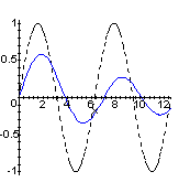
Evaluating an expression like with(plots) loads commands defined by the named package. You will probably find those defined by the plots, DEtools, linalg and orthopoly packages most useful at first.

Sample Applications

Energies of the Particle States in a Finite Square-Well Potential

This simply illustrates the power of the strategy of plotting expressions, visually searching for solutions to an equation or system of equations and then using fsolve to refine your estimate of the solutions.

In Quantum Physics Gasiorowicz shows that the energies of even parity states of a particle of mass m in a square-well potential of depth -V0 that extends from x = -a to x = a can be determined by solving the equation

> Eeq := tan(y) = sqrt(lambda - y^2)/y;

where y = q a is the rescaled magnitude of the particle's momentum within the well and .

The following plot shows that there are two even parity states when has the value 25.

> P1 := plot(sqrt(25-y^2)/y, y=0..2*Pi, 0..10, color=black):
> P2 := plot(tan(y), y=0..2*Pi, 0..10, color=blue, discont=true):
> plots[display]({P1,P2});

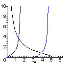
The y values that determine the energies of the two states are

> fsolve(subs(lambda=25,Eeq), y, 1..1.5);

> fsolve(subs(lambda=25,Eeq), y, 3.2..4);

Lagrangian Mechanics and the Pendulum

Consider a bob of mass m = 1 kilogram that swings freely in a vertical plane at the end of a rigid, massless rod of length l = 1 meter.

To illustrate the slick way in which Maple can handle Lagrangian mechanics the analysis that follows begins by representing the bob's motion using Cartesian coordinates in the vertical plane and shows computations step-by-step. Note that the computation of Euler-Lagrange and Hamilton equations is easily automated.

Let x denote horizontal displacement of the bob from the pendulum's point of suspension and y denote its vertical displacement measured down from the suspension point.

The following defines a few commands that facilitate Lagrangian computations.

> read `a:fdiff.mpl`;

Once this file is loaded, you can indicate that the particle's x and y coordinates depend on time as follows

> depend({x,y}, t);

and can enter first and second derivatives of these functions using the concise notation

> dx, ddx, dy, ddy;

This makes entering the expression for the particle's kinetic energy a snap.

> T := (m/2)*(dx^2 + dy^2);

The corresponding potential energy and Lagrangian are

> V := -m*g*y; L := T - V;

If the functions x and y are treated as independent generalized coordinates, this Lagrangian produces the equations of motion that govern projectile motion. It leads to the pendulum equation of motion only when the holonomic constraint imposed by the massless rod that suspends the bob is accounted for. This is most easily done when using polar coordinates as generalized coordinates in the plane. The transformation to a convenient set of polar coordinates ( = 0 when the bob is directly below the suspension point) is easily accomplished by

> depend({r,theta},t):
> x := r*sin(theta): y := r*cos(theta):

With these assignments made Maple's full evaluation automatically makes the coordinate transformation for you.

> L := simplify(L);

The assignment

> r := l;

imposes the constraint in the same automatic way.

> L;

The pendulum equation of motion is this Lagrangian's Euler-Lagrange equation

> DE := diff(fdiff(L,dtheta),t) = fdiff(L,theta);

When values for the parameters appearing in this equation are assigned and initial conditions specified you are ready to use Maple's numerical capabilities to simulate pendulum motion.

> m := 1: l := 1: g := 9.8:
> ICs := ic(theta,t=0,1), ic(dtheta,t=0,0);

The following Maple command assigns the name Sol to a procedure using an adaptive Runge-Kutta algorithm that Maple creates to estimate this motion.

> Sol := dsolve({DE,ICs},theta,numeric);

Such procedures return estimates in an odd format,

> Sol(0); Sol(0.5);

but Maple provides special plotting commands to handle this sort of output. The following plot

> with(plots):
> odeplot(Sol, [t, theta], 0..3, color=black);

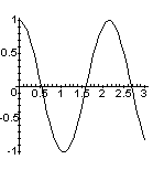
shows the pendulum's displacement as a function of time while this one

> odeplot(Sol, [theta, dtheta], 0..3, scaling=constrained, color=black);

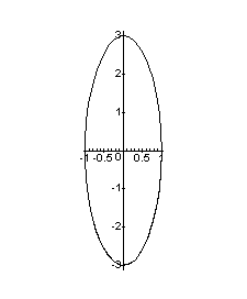
shows its trajectory in phase space.

Here is one way to define functions that directly return the values of the pendulum's angular displacement and its angular velocity.

> TSol := a -> subs(Sol(a), theta):

> dTSol := a -> subs(Sol(a), dtheta):

> TSol(0), dTSol(0.5);

These can also be used to produce graphs like those above and many others.

Here, TSol is used to estimate the pendulum's period as an alternative to evaluating the usual integral representation of this quantity.

> 4*fsolve('TSol'(t), t=0..1);

Remember that this depends on the pendulum's angular amplitude, in this case 1 radian.

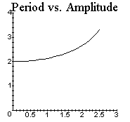
The following uses this brute-force method of determining the period to produce a plot of period versus angular amplitude for the range of amplitudes from 0 to 2.5 radians.

> for i from 1 to 25 do
> ICs := ic(theta,t=0,i/10),ic(dtheta,t=0,0):
> Sol := dsolve({DE,ICs},theta,numeric):
> P.i := [i/10, 4*fsolve('TSol'(t), t=0.41..1.0)]:
> od:
> P0 := [0,P1[2]]:
> plot([seq(P.i, i=0..25)], color=black, view=[0..3, 0..4], title=`Period vs. Amplitude`);