Quantum Percolation: Electrons in a Maze
Physicists, especially theoretical physicists, love to make models of the world to help us understand it. We weigh various effects against each other, pick out key features, make simplifying assumptions, and reduce a physical phenomenon to its simplest, most tractable mathematical description to get an approximation to reality. Then, bit by bit, we add layers to our mathematical models to create a richer, more complex, and more accurate description of what we observe. While this approach sometimes makes us the brunt of good-natured jokes (“assume a spherical cow…”), our method nonetheless has considerable value. The physical world is incredibly complex, and it is by joining our models with experimental studies that we physicists are able to explain “why the world does what it does” and make predictions about new phenomena not yet observed.
One simplified model is the quantum percolation model, which helps physicists understand electrical conduction. Physicists identify two key factors in electrical conduction: the interactions between electrons (they repel each other), and the disorder of the underlying material (e.g., impurities). The quantum percolation model is one of a few models that look only at the effects of disorder (or randomness) on conduction. This is, admittedly, where the model is simplified - in reality, a material has many electrons, so interactions between them will be important. However, the idea is that by ignoring interactions, we can get a better grasp on the role disorder plays in conduction. Once we have done that, we can combine the disorder-only model with one of the interactions-only models for a more complete picture. The quantum percolation model is particularly interesting because the electron behavior it models in two dimensions contradicts the expectations that were set forth by physicists studying a different disorder-only model, the Anderson model. In 1979, E. Abrahams and his colleagues used a mathematical method called scaling theory to predict that even a very small amount of disorder in a two-dimensional system would destroy conduction and make the entire system become insulating (Phys. Rev. Lett. 42, 673). From the electron’s perspective, this meant that the electron would always be localized (confined to a small area), as opposed to being delocalized as it would be in a conducting material. The scaling theory prediction proved true for the original Anderson model, which is why electron localization due to disorder is often called Anderson localization. It was initially expected that the scaling theory result would be valid for other disorder-only models in two dimensions, but as we will discover, adding disorder in the quantum percolation model does not always result in electrons being localized.
To understand the quantum percolation model, we first need to take a step back and look at the classical percolation model. The word “percolation” might remind you of coffee-making, and there’s reason for that! “Percolation” simply means the process of one substance passing through another substance that has many holes in it at random locations. Much as the water in your coffee pot must find a way through the spaces between coffee grounds to make your morning coffee, a particle in the percolation model must find a path through a lattice of points that has many empty sites (holes) in it – the only difference being that in the percolation model, the “holes” are what impede transmission, not allow it. This type of percolation, with some sites removed, is called site percolation; alternatively, we could remove links between sites instead, which is called bond percolation (see Fig. 1a and 1b). In both cases, the only way a particular lattice can transmit a particle is if there is a connected path between the start point and the end point (for instance from the upper left corner to the lower right corner in Fig. 1), just like a maze. If we dilute the lattice too much, there won’t be any transmission – all possible paths from the start point will lead to dead ends! For classical percolation on a square lattice (i.e. a square grid of points), this occurs when we’ve removed 41% of sites (in site percolation) or 50% of bonds (in bond percolation). Of course, even for dilutions less than that critical percentage (qc ), say, at only q=10% sites removed, it is possible to get a particular arrangement that has only dead end paths between our chosen start point and end point. However, on average for all different ways of arranging a q<qc dilution, we have a non-zero chance that our chosen input and output will be connected and a 100% chance of finding some connected path across the lattice (while not necessarily between the two arbitrary points we chose), meaning the lattice is conducting. For q > qc there is zero chance of finding a connected path across the lattice no matter what two start and end points we choose, therefore the lattice is insulating.
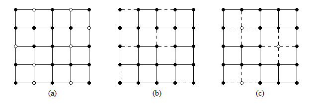
Figure 1: Example lattices for (a) site percolation (b) bond percolation, and (c) the modified site percolation used in our study.
Quantum percolation modifies the classical percolation model in one small but very significant way: instead of sending an ordinary particle through the lattice, we use a quantum-mechanical particle, in this case, an electron (though we ignore many electron properties because of our model being a simplified one). You may know that electrons exhibit particle-wave duality, that is, they have the properties of both particles and waves. It is the wavelike nature of electrons that makes the quantum percolation model more complex, because the electron wave function can interfere with itself, analogous to how light interferes with itself to create a pattern of light and dark spots when shined through two very narrow slits (Young’s double-slit experiment). This characteristic means that the electron may not be transmitted even when a connected path is present on the lattice, since its wave function can reflect off of the infinite-energy barriers created by the removed sites/bonds, resulting in the electron interfering with itself (just like a wave of water interferes with itself when reflecting off a wall). Because of these interference effects, we expect that the critical dilution above which there is on average no transmission will be a lower dilution than in the classical percolation model.
In our study of the quantum percolation model, we look at a modified version of site percolation: at a given dilution q, we randomly remove q% of the sites on a square lattice with NxN sites, and as we do so we also remove the four bonds connecting that site to its neighbors, since an electron on one of those neighbors now has nothing to hop to (Fig 1c). By removing the site, it’s as if we have put an infinitely tall wall around it; no matter how much energy an electron has, it can’t get over the walls to get to that site. Thus, as the electron spreads across the lattice, whenever part of its wave function encounters a diluted site, that part is reflected back, while the rest of the wave function continues on through the lattice. At low dilutions, the disordered lattice is like a room with scattered infinitely-tall pillars – only a small part of the wave function will be reflected overall. At high dilutions, the lattice is like a maze with many twisting corridors and dead-ends – there will be much more reflection and interference, enough that the chance of the electron getting through is very low (if not zero) even if there is a connected path across the lattice. Having diluted the lattice, we send an electron with some energy E into the one corner of the lattice, and, using a combination of quantum mechanics and computational methods, we calculate the electron’s transmission through the opposite corner. We repeat the process several hundred times for different realizations of the NxN lattice (that is, different ways of arranging the q% diluted sites) to get the average transmission for that lattice dilution and electron energy.
To establish whether the electron is delocalized at a given dilution q and energy E, however, we must measure not just the average transmission, but also the average transmission on different sized lattices, in order to scale up to a macroscopic system - physicists call this the thermodynamic limit. After all, even just a nanogram of matter contains trillions of atoms, so a 100x100-atom lattice is not very realistic! Starting with a lattice of just 10x10 sites, we calculate the average transmission over successively larger lattices, up to NxN with N≈900. We then plot the average transmission T vs the lattice size N to determine the trend as N→∞. If the transmission eventually levels off to some non-zero value, we know that the electron is delocalized. If the transmission decays to zero, the electron is localized; how quickly the transmission decreases tells us whether the electron is strongly or weakly localized, i.e. whether it is stuck in a very small area of the lattice or is spread over a somewhat larger area that is still small enough to keep the electron from travelling across the lattice.
So far we’ve discussed these calculations in general terms: some energy E, a given dilution q. In actuality, we calculated the average transmission for six electron energies E and about a dozen dilutions q between 2% and 38%. Combining the results for all energy and dilution pairs gives us a phase diagram for the 2D quantum percolation model (Fig 2). The phase diagram tells us that, within the energy range we studied, it is in fact possible to have a delocalized electron state for low dilutions. This discovery suggests that disorder does not always prevent conduction in two dimensions, in contrast to the Anderson model results (the other disorder-only model) and the scaling theory predictions! Instead, the relationship between disorder and conduction in two dimensions is more complex. Disorder has a stronger effect at smaller energies, as seen by the decrease in the phase boundaries for E<0.1, a result which is consistent with previous related studies. Additionally, as disorder increases, there is not an abrupt shift from delocalized to strongly localized, but rather, there is a region of weak localization between the two for all but the smallest energies. For all energies, our results indicate that the critical dilution at which the electron is always strongly localized is in fact lower than the classical percolation threshold for zero transmission, as we predicted.
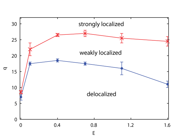
Figure 2: The dilution q vs energy E phase diagram for the quantum percolation model, showing the phase boundaries between the delocalized, weakly localized, and strongly localized phases that the model exhibits.
Having established that disorder does not necessarily prevent conduction in the two dimensional quantum percolation model, an interesting question to consider is how important it is for the diluted sites to be completely disconnected from the rest of the lattice, or, in physics terms, what happens if we introduce the possibility of tunneling. When a classical particle encounters a barrier, it is reflected unless it has enough energy to go over that barrier. For a quantum mechanical particle like an electron, complete reflection only occurs for infinite energy barriers. For finite barriers, it might be reflected, but there is also some probability that it could be transmitted through the barrier instead, which is called tunneling. We can introduce the possibility of tunneling in our model by making the bonds attached to diluted sites weaker than available-site bonds, but not completely nonexistent as in the original model. This gives the quantum percolation model a parameter for diluted-site bond strength, which we call w, that has values between 0 and 1. For w=0 (no bond) the model is the same as the regular quantum percolation model; for w=1 (full bond) the model is the same as a perfect fully-connected lattice. For 0 < w < 1, diluted sites all have the same bond strength that is some fraction of the available-site bond strength w=1, meaning they are still partially connected to the other sites and the electron may be able to tunnel through the diluted sites. Using the maze analogy, it’s as if we have changed the infinitely tall walls around the diluted sites into finite walls ranging from very very tall (small w, similar to the w=0 case) to short shallow bumps (large w, similar to an ordered lattice). Our intuition is that at higher values for w, the modified quantum percolation model will behave similarly to a perfectly ordered system, with no localized states, but we are unsure of how quickly the model’s behavior will change when increasing w from 0. If completely disconnecting diluted sites is what gives the quantum percolation model its characteristic three phases, we expect to see localized states eliminated for even small w when we introduce tunneling by making the diluted site bond strength nonzero. If having a binary disorder (that is, having two bond strengths, one for available sites and one for diluted sites) is the more important aspect of the quantum percolation model, we expect to see the localized phases persist for some range of w.
To study our modified quantum percolation model, we perform the same calculations as described for the original model, but repeat the process a few dozen times for different values of w. Everything except w is the same for each round – we use the same six energies, the same lattice sizes, the same dilutions, and even the same sets of disorder realizations! This ensures that any changes observed in the model’s behavior are truly the effect of changing the diluted site bond strengths. Having done this, we organize our results into phase diagrams showing the effects of bond strength w and dilution q for each of the six energies studied. The phase diagrams for three of those energies are given in Fig. 3. Two features stand out in these diagrams. First, for the larger two energies, the phase boundaries are level at least to w=0.05, and even up to w=0.3 for the largest energy. It is surprising that we can make such a substantial change to the model without seeing any quantitative change in its behavior! In fact, even though the phase boundaries shift as we increase bond strength, the three phases characteristic of the quantum percolation model persist; the localized states do not disappear completely for all energies until the bond strength is just over half of its maximum. Again, the model’s behavior is surprisingly stable! These results suggest that having a binary disorder is much more important than having the diluted sites isolated from the rest of the lattice. The second interesting feature is that the lower the energy, the more rapid the change in the phase boundaries as w increases. In fact, for the smallest energy, E=0.001, increasing the bond strength to a mere w=0.01 (100th of the maximum strength) tips the system into wholly-delocalized states for q<14% (we did not study q>14% for this energy because it was computationally expensive; E=0.001 calculations are very slow). We are not entirely certain why the quantum percolation model is more susceptible to small changes at low energies, but the result is consistent with the original model’s behavior, in which localized states appear for smaller dilutions than all the other energies.
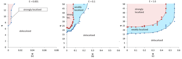
Figure 3: Dilution q vs bond strength w phase diagrams for the modified quantum percolation model at (a) E=0.001, (b) E = 0.1, and (c) E=1.6
In the end, what does our study of the two-dimensional quantum percolation model tell us? First, it defies expectations for two dimensional systems by actually allowing delocalized states at low disorder, instead of even a small amount of disorder in the system automatically destroying conduction. Secondly, the phase characteristics of the quantum percolation model appear to depend predominantly on the disorder being binary, rather than the strength of the connection between disordered and ordered sites. This makes the quantum percolation model applicable in a wider variety of situations than its original form, such as situations in which it might be unrealistic to model the disorder (such as impurities in a material) as completely isolated from the rest of the material. In the future, the modified model discussed here will need to be further modified to account for interactions, allowing it to be applied to even more situations. However, even in its highly simplified form, we have found that quantum percolation can give us a rich picture of the role disorder plays in determining electrical conduction.
Brianna Dillon-Thomas, PhD 2016